Processing Oblique UAS Imagery Using Image Annotation

Introduction

       In previous labs throughout the semester the imagery used has been in a format called nadir. Which is when the camera is at a position that it is pointing directly down, meaning the location of the images is above the target. A camera pointing to the nadir direction means that it is vertical or perpendicular to the ground. Nadir imagery is used for creating orthomosaics and digital surface models using Pix4D.
      In this lab, the aerial images used that were were oblique imagery. Oblique imagery is aerial photography that is taken at a 45 degree angle from the ground or the object that is the subject of the flight. The 45 degree angle enables users to be able to measure the entire object, rather than just the top of the object as in nadir imagery. Using oblique imagery is applicable in the geospatial market because it allows for the creation of 3D models and it allows for measurements of the sides of structures along with the top. Oblique imagery is used in urban planning, crisis management, and it also has a variety of other applications.

Methods

        The purpose of this lab is to use a process called annotation in Pix4D to get the fundamentals regarding processing and correcting oblique imagery. Image annotation is used to remove all the discrepancies around an object so that the subject of the imagery is more accurate. After the initial processing in Pix4D is complete the annotation toolbar can be accessed by clicking on the ray cloud and then selecting an image on the left hand side for annotation. Next click the pencil icon on the right hand side which will allow the user to begin annotation. Make sure the annotation method is mask, then the entire image was annotated by clicking on the areas that were not what was wanted for the 3D model. After everything by the target is annotated, click apply and repeat the process until all angle are covered. After the number of images annotated is sufficient, be sure to click the advanced tab under processing options and the use annotations tab under point cloud and mesh. Then uncheck initial processing and select the point cloud and mesh and process the data with annotations. After completion turn off the cameras and click on the triangle mesh tab, this will generate the 3D model. The same process described above was used for all three image sets.
         There are three types of annotation that can be used, mask, carve, and global mask.  In this lab the mask form of annotation was used. Mask annotation removes the background around the subjects. Not every image needs to be annotated because there is considerable overlap between the images. Throughout this lab three different oblique aerial image sets were used in an effort to create 3D models of each. The initial images were processing with and without the annotation to see if there were significant differences.
        After Pix4D is open the first image set was added, the work space was set up correctly and the camera model was changed to linear rolling shutter. From there the model that was selected was the 3D model. This is important to note because in previous labs the 3D map was used, if the 3D map is selected the processing will be very slow and there will be errors when trying to begin the annotation process. This change is done because there will be no orthomosaics or DSM's created, but rather a 3D model the shows all the angles of the subjects of the flight.
         The first image set that was worked with was a bulldozer that was located at the Litchfield Mine to the southwest of Eau Claire. The second imagery set that was used was a shed that is located on the property of Eau Claire South Middle School. The third imagery set is of Professor Hupy's now retired Toyota Tundra in the parking lot near Eau Claire South Middle School parking lot. Each of these oblique imagery sets were taken by a DJI Inspire, the UAV flew in a tornado pattern around the subjects, in an effort to capture all angles of all sides. Figure 1 below shows how the drone was flew in an effort to cover all of the angles. The flight for the truck is shown, though the other two flights looked much the same. Each image set will be described in more detail below.

Figure 1: Flight Pattern

Bulldozer

         Figure 2 below shows an annotated image of the bulldozer at the Litchfield mine. It is easy to see all of the little spots that are indented on the bulldozer, these are hard areas to get accurately, though as shown below it can be done.

Figure 2

Shed at South Middle School

       Figure 3 below shows an annotated image of the shed at south middle school. The white dashes at the bottom of the image can be tough to get so be sure to zoom in, also the shadow on the left of the image need to be done carefully, as the software may consider the shadowed part of the building the same as the shadow on the ground.  

Figure 3

Pickup Truck

         Figure 4 below shows an annotated image of the Toyota Tundra that was done in a parking lot. Make note of how hard the tires are to annotate and be sure they are done accurately, also be sure the bumper and mirrors are not selected as they are important to making an accurate 3D model.

Figure 4

         The rematch and optimize tool was used on each of the data sets to see if that would better the results. The conclusion that made was that the rematch and optimize is not necessary as there was no notable improvement. Also this process can take some time depending on the size of the image set, so there was no need for the wasted time with this additional step.
        After spending many hours doing the annotation process a few tips can be offered. Making circles is an effective way to cover a lot of ground. Also clicking and holding the cursor means the annotation process in continuous. Start at the outside of the image and work in, be careful not to get to close to the object when holding the mouse because a large part of the object could get selected and then the eraser will have to be used.


Results

          Below are screen captures that show multiple angles of each of the image sets. Each one will be discussed in more detail individually. Ultimately each image set still had flaws from the background of the images, and that will be discussed below. In these setting the image annotation was still morphed from the background, though the tool set of being able to eliminate the backgrounds of images for 3D model creation is an essential tool to have. Also one of the first things to be done right before annotation is to increase the size of the box used for annotating. This helps creates larger pixels and makes the process go much quicker.

Bulldozer

        The bulldozer was by far the most challenged image set to annotate. There was a lot of nooks and crannies that are very challenging to annotate correctly. This was the first set that was done, and that was done because this was the trial run to get a feel for how things worked. Five images were annotated here. Figures 5-7 are the output images after the annotation and figures 8 and 9 show the bulldozer with no annotation. The differences are not notable, even on closer inspection, zoomed very far in there are minuscule differences at best. This is unfortunate to see due to the time that was spent annotating.

Figure 5: Annotated

Figure 6: Annotated

Figure 7: Annotated

Figure 8: Not Annotated

Figure 9: Not Annotated

Shed at South Middle School

         The shed at south middle school went quite a bit smoother and faster than the other two data sets. the shadows that were cast caused a few issues, and also the lines on the track and the fence posts were hard to get at some points, that can be remedied by zooming in, but not zooming in so far that the software breaks up the smaller areas into tiny pixels. For this image set 15 images were annotated because the process went very quickly. Along with increased annotation, the rematch and optimize was done to see if the output quality would be better. By doing more images, one would believe the quality would increase, again, unfortunately there was not a lot of improvement from the images with no annotation. One difference that can be noted is that were is less of a pix elated look on the annotated image. Though the there is still the error on the peak of the shed. Also the sides are a little more clear on the annotated image.

Figure 10: Annotated

Figure 11: Annotated

Figure 12: Annotated

Figure 13: Not Annotated

Figure 14: Not Annotated

Pickup Truck

         Annotated the Toyota Tundra was slightly more difficult than the shed at south middle school but not nearly as tough as the bulldozer. The mirrors and fender flares caused some issues as the software had a difficult time differentiating between the ground and those objects, also the bumper kept wanting to be selected when it was not supposed to be. Again, just the same as the two previous data sets there was not a notable difference from the image set that was annotated and the one that was not.

Figure 15: Annotated

Figure 16: Annotated

Figure 17: Annotated

Figure 18: Not Annotated

Figure 19: Not Annotated

Conclusion

          After completion of this lab it would be easy to assume that annotation of oblique imagery is not necessary, though most of the time it is. All in all it certainly does not hurt the quality of the data set and any improvement of data quality that can be done should be. Oblique imagery does a nice job of creating a 3D model of structures. After completing this exercise it would be recommended that if a large image set needs to be annotated the job could be outsourced to a different company. This is due to the large amount of time that it takes to do the annotations and the fact that it can be very stressful when things get annotated that were not intended to get annotated. Other issues with annotation were the shadows, clouds, and little objects such as the dashes on the track at south middle school, the mirrors and fender flares on the truck, and most of the dozer because there was not many straight lines, but rather a considerable amount of intents that had to be dealt with. When annotating it was found that it is important to do images from each angle around the subject being annotated. Doing this will cut down on the number of images that need to be annotated because there will be alot of overlap with other images if the angles selected are correct. Also for whatever reason some images just do not cooperate, if an image is being hard to annotate it is recommended to just try a new image.

Sources

https://pix4d.com/support/

Calculating Volumetrics Using UAS Derived Data

Introduction

          Volumetric Analysis is the study of volumes of objects using aerial imagery. Volumetric Analysis is used often in Unmanned Aerial Systems, as well as in other aspects of geography such as remote sensing. This application has many uses, it can be used to calculate the volume of anything from buildings to natural features.It is important to note that in order to do this analysis x,y and z values are needed to get an accurate measurement. The images used throughout this lab were captured by a DJI Phantom 30 and they were collected with high overlap, allowing for the creation of a Digital Surface Model. The use of ground control points in this lab also adds to the accuracy of the volumetric analysis. To the southwest of Eau Claire is the Litchfield Mine site, this location has been used in several exercises during the semester. For this lab three sand piles were selected at random and a volumetric analysis was completed on them using Pix4D, 3D Analyst and by running a TIN. There was a number of tools used in this lab including the volumes tab in Pix4D, the extract by mask and surface volume tool for 3D analyst and finally the Raster to TIN, Add Surface Information and Polygon Volume for the TINs. After the calculations were done using three different methods a table including the three values and there averages was generated along with multiple maps.

Methods

        The first method used was the volumetric analysis in Pix4D. The project that was used in lab 5 which was the Litchfield Mine with GCP's was used. On the far left under the Volumes tab the user can draw points around the sand piles and by simply clicking calculate the volume of the pile in meters cubed is provided. 

Figure 1

           Figure 1 above illustrates the three piles that were used in this lab. The pile on the far right is pile 1, pile 2 is in the upper left hand side and pile 3 is pictured on the bottom right. Volumetrics is interesting because upon an initial glance pile 2 looks to be the largest, though pile one is significantly larger in actual area, and that will be discussed further in the results section. Figure 2 shows that pile 2 is more than a third smaller than pile 1. This is a very fast method to get the volume, it is efficient and very accurate.

Figure 2

         The second and third methods used to calculate the volume of the sand piles were both in ArcMap. There are other ways as well, but for the purposes of this lab two were selected, being 3D Analyst which calculates using the digital surface model and TIN, which is done by creating a TIN from the surface. First a new geodatabase was created and there were three feature classes created that were used for piles 1,2, and 3. Next using the editor tool bar polygons were created of each sand pile. Next the Extract by Mask tool was used to clip the areas that were just created from the DSM. Next the Surface Volume tool was used to get the volume of the sand piles.

         The third and final method used was the use of TINs's to calculate volume. The clips that were made in method two were used in the Raster to TIN tool which was found in the ArcHelp search bar. A TIN is generated from the raster, from there the Add Surface Information tool was used to get the elevation values for the TIN. After running the Add Surface Information tool a new layer is created in the results tab on the far left, after adding the layer to the map, the volume values are available by looking at the attribute table. The final step here is to use the Polygon Volume tool, this tool uses the TIN and the value that was just recorded in the previous step.

Results

          Figure 3 below is a table that displays the different volumes recorded for each pile along with the average of each method. Each of the methods are reasonably close to each other. The 3D analyst and TIN values were significantly closer that that of Pix4D, this can be easily explained by the fact that the data in ArcMap came from drawing polygons again, so there was a slight variability from Pix4D. When looking at pile three, there is not much difference between the three, this is because that pile was very symmetric, it was nearly a perfect circle, whereas piles 1 and 2 were very irregularly shaped. Another factor that would account for piles 1 and 2 having a greater variability is the fact that they were much larger, therefore there is more room for error when drawing the polygons.

Figure 3

         Figure 4 below is a map showing the changes in elevation of each of the piles. Each pile has a peak, which makes sense because that is how sand piles are made. Pile 1 is purple, pile 2 is red and pile 3 is purple at there highest elevations. This is important to note that pile 2 appears larger than pile 1, though pile 1 is over 400 meters cubed larger than pile 2. Those values are clearly depicted above by figure 3.

Figure 4

          Figure 5 below is a map that shows the full extent of the Litchfield mine to give perspective to the size of the pile compared to the overall size of the mine. As talked about previously, pile 2 had much less volume than pile 1, though they appear nearly the same size. Pile 3 was very small as it was over 55 times smaller than pile 1.

Figure 5

Conclusion

          After completing this lab it is easy to see all of the applications of volumetric analysis. The ways that were used in this lab were just three of the many ways these calculations can be done. Without question Pix4D is by far the quickest method, there is no actual baseline of what the actual sizes of the piles are, so it is not possible to tell which method was the most accurate. The TIN and 3D Analyst both used the same polygons that were drew, and calculated values using the same DSM, this accounts for there similarities at least in part. Even the slower methods of volumetric analysis are much faster than a company paying for someone to manually collect these values. 

Processing Multi-Spectral Imagery

Introduction

          The Micasense RedEdge 3 is a multispectral camera that can capture 5 different bands all at the same time. The bands being capture simultaneously are the red, green, blue, RedEdge and near infared (NIR) bands. The imagery used in this lab is from a RedEdge sensor. Before getting into the methodology and results of this lab it is essential to have a little background regarding the RedEdge sensor. The camera has a lens focal length of 5.5 mm and a lens field of view of 47.2. The image sizes are 4.8 mm by 3.6 mm and the resolution is 1280 x 960 pixels. A standard RGB sensor only has red, green and blue, whereas the RedEdge boasts the RGB along with NIR and RedEdge. It is essential to take note of the proper order of the bands which is blue, green, red, RedEdge and NIR. The addition of the RedEdge and NIR allow the user to have very precise quantitative data regarding the type and healthiness of vegetation. The ultimate goal of this lab is to process imagery captured from an unmanned aerial system and to then classify whether the land use is pervious or impervious.

Methods

          The image set used for this lab was very large, so a good amount of time was allotted to allow the files to copy over from the share folder, the images were provided from Professor Joseph Hupy. Once the data sets were copied over a new project was opened in Pix4D. From here Figure 1 below shows how the new project was named, the name included the data the images were processed, the location of the images and the type of sensor that was used as well. .  The file was saved in a location dedicated to this exercise and using a name that tells the user everything they need to know about what is in the folder.

Figure 1

   

           Figure 2 illustrates a one of the few changes that had to be made before the data could be processed. In previous exercises 3D maps were created, but for the purposes of examining land cover, a Ag Multi spectral template was selected. The RedEdge is compatible with this template as shown on the right side. By using this template there will be no Raster DSM or Orthomosaic Geotiff.

            A few of the processing options needed to be changed before the data could be processed. The Geotiff with transparency box was check, as there was issues when it was left unchecked. From here the processing was ran much the same way as was went through in detail in the previous two labs.

Figure 2

           Figure 3 below shows the amount of overlap that was in the images after processing the images in Pix4D. It is clear there is a sufficient amount of overlap on 80% of the flight, the area that is being examined close has good overlap.

Figure 3

         Figure 4 is the quality report, this is always provided as it gives the viewer an idea of the quality of the data. Only 69% of the images were calibrated, this was explained in Pix4D by looking at where the pictures were taken from, as the drone was taking off there were many images on the way up that were not used because they had no benefit.

Figure 4

             Figure 5 below shows a summary of information about the area covered and the data it was processed as well as the band used in this particular flight shown below. The camera model names are all shown clearly, the blue, green, red, RedEdge and NIR. The second to bottom row shows the amount of area that was covered in the flight, that being 6.904 acres.

Figure 5

          After the processing was completed in Pix4D there is a Geotiff for each of the five bands. For use in this lab the bands needs to be brought together as one composite band. This was done in ArcMap using the composite tool under the help menu. After all five bands were added as the input, a output location in the same folder used in the Pix4D processing was selected. Once a composite was made the layer was copied three times in order to ensure there is three different combinations of bands that each display something different. This is where is it essential to make sure the bands are in the correct order, the correct order being blue, green, red, RedEdge, NIR. Changing the order of the bands allows for different bands to be the center displayed.


Results

          Below are maps showing RGB, Near Infared, and RedEdge, below that is a map showing what areas of the flight are permeable and impermeable. Each of the figures 6-8 has the bands arranged in different ways as shown in the legends and that accounts for the variability in each.

Figure 6

          Figure 6 above is the closest of figures 6-8 to an orthomosaic, though there is a slight influence from the red band that shows up as a purple color on the map. Vegetation shows up much the same as it would on an aerial image, the healthy vegetation is a dark green while the unhealthier vegetation seems to appear more brown. The road on the west side of the map runs north to south and the driveway to the house runs west to east. The main structure in the map is almost center and the structure is a house.

Figure 7

           Figure 7 above illustrates the false colors generated from a near infrared band. The healthiest vegetation is shown by the darker shades or orange as shown to the east of the house. When comparing the field to the north of the house it is clear how sparse and unhealthy the vegetation is compared to the area east of the house. 

Figure 8

         Figure 8 above does a fantastic job of illustrating what areas are healthy vegetation and what areas are not. The road on the west side of the map is shown clearly, along with the drive way. The healthy vegetation to the east of the house can be shown very distinctly by a dark red/pink. In comparison the area to the north of the house that looked unhealthy in figure 7, it now is shown here that the vegetation is in fact healthy. In contrast the southern third of the map is a very pale color rather than a dark red. Around the house a large majority of the yard is shown dark red, most likely this can be assumed because the homeowner most likely waters there yard.

Conclusion

            This lab required the knowledge of both Pix4D along with ArcMap and ArcPro. By processing multi-spectral imagery gathered by the MicaSense RedEdge Senser the type of land use was able to be determined. Each band has its own benefits and the use of both Pix4D and the Arc programs together helped to showcase the skills learned throughout this course. Sensors such as the RedEdge are designed for use in the Agriculture department and they can be used in a similar fashion to this exercise in order to see what areas of vegetation are doing good and what areas are not. This has uses in the commercial and residential levels. Value added data analysis coupled with UAS data allows for the user to see what areas are doing well and what are not, the UAS data allows for accurate imagery with the sensors.

Processing Pix4D Imagery with GCP's

Introduction

        This lab was done almost identically to the previous lab, as it dealt with processing the same data in Pix4D, though this time there was an addition of ground control points (GCP's). The addition of GCP's helps ensure data integrity. In order to understand why GCP's are significant, they first need to be understood. Ground control points are a specific location on the earth's surface that was placed there by the operator flying the area in an effort to be able to tie images down to the earths surface. Each ground control point has a coordinate on the earths surface assigned to it. GCP's are used by drones, satellites, and airplanes and they are used to georeference the data that was taken during flight. As discussed in the previous lab, GCP's are not required when working with aerial imagery if the location of the images is known, but if the aerial images are not geolocated then GCP's must be implemented. Even when the images are geolocated they can still be off by tens of meters so the use of GCP's when possible is encouraged. In this lab a brief summary of running Pix4D will be discussed as well as the methods used to tie down the GCP's will be walked through. The initial processing will be re optimized after the GCP's have been tied down.  In the end the goal is to determine the difference in data quality from aerial imagery with GCP's and aerial imagery without GCP's. 

Methods

          For this lab a new project was created in Pix4D, name the same way as the previous lab, except this time the GCP's were added to the end to show that GCP's were used. The initial directions for this lab instructed to run the Litchfield flights 1 and 2 separately. After running them separately there was issues with the merge and with the GCP's, most definitely user error, so the second time the flights were brought in together, which did add a significant amount of time to the process. Though this way took longer, there was no longer the step to merge and the data processed with no issues. In total there were 155 images brought into Pix4D. The steps in this lab were done almost identically to the previous lab. Be sure to change the camera mode to linear rolling shutter, as shown by figure 1 below. Next, under the "DSM, orthomosaic and index", which is tab 3, be sure to change the raster DSM method to triangulation rather than inverse distance weighting.  The default coordinate system is acceptable for use here so leave that at WGS1984(egm96).

Figure 1

          The next step is shown below by figure 2. Under the project tab, there is a GCP/ MTP manager that allows the user to import GCP's. After clicking on import GCP's the screen below will pop up, the coordinates order is changed to Y, X, Z rather than X, Y, Z because Y is the false easting, X is the false northing, and Z is the elevation. If it is left in X, Y, Z the GCP's will not import in the correct locations.

Figure 2

Figure 3

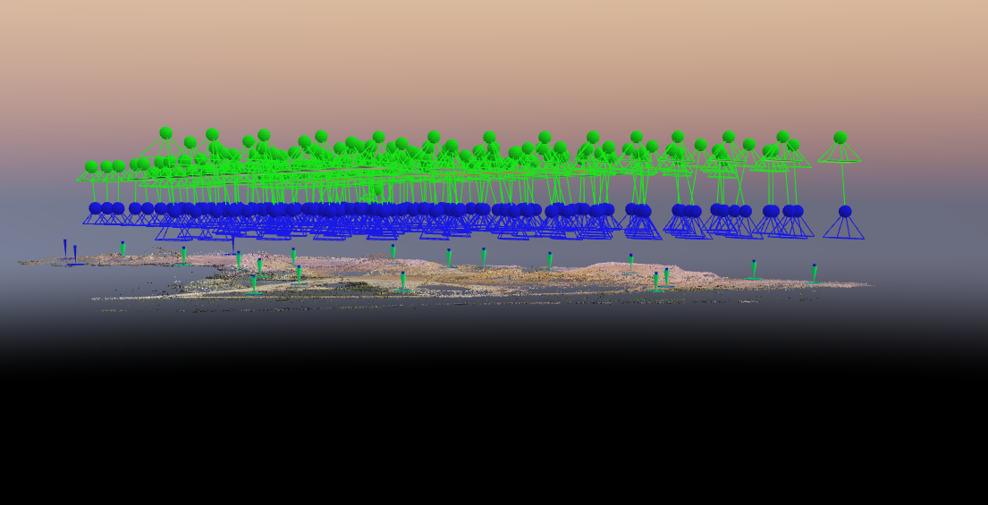
        Figure 3 above shows where the images were taken from both flights 1 and 2. The blue X's mark the locations of the GCP's. All but 2 of the GCP's were tied down, for two of them they may have been moved or accidentally covered up. Before the initial processing was ran, the GCP's were tied down using the basic editor in order to make the initial processing more accurate and to make the later steps using the ray cloud easier. 

Figure 4

          After the initial processing was complete, the rest of the images were tied down using the rayCloud. Figure 4 above shows that the GCP's had to be tied down in every image they were visible in. This was done by zooming into the correct GCP and placing an "X" on the center. This is the process of georeferencing, using a point with a known coordinate to make the aerial imagery more accurate. After all of the GCP's were tied down for every image they showed up in, the imagery was then reoptimized.

Figure 5

         Figure 5 shows the imagery after reoptimizing for both flights 1 and 2. There was only 3 GCP's that remained blue and they did so because they did not show up in any of the images taken. As stated earlier this could be because they were moved, or accidentally covered up. The green points that are on the surface are the GCP's that were correctly tied down and reoptimized. After this step is complete, uncheck box 1 next to initial processing and check boxes 2 and 3 and press start. The final product of all the processing is a very high quality orthomosaic and DSM that can be used for map making in ArcMap.

Figure 6

Figure 7

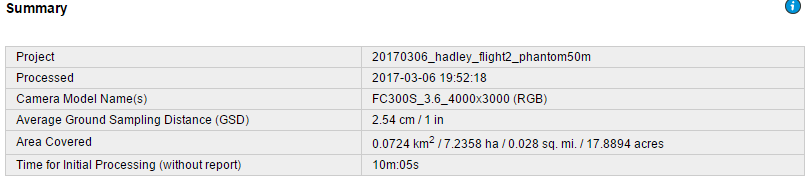
         Figure 6 and figure 7 above show a few snippets from the quality report that is received after processing. Figure 6 shows that 155 out of 155 images were calibrated and that there is georefrencing. The summary shows what the project was called and when the data was ran.

Results

         In the results section there will be comparisons made between the Litchfield mine with GCP's and without. This will be done in an effort to determine if the GCP's are really worth the extra time. Figures 8-11 are maps generated from the aerial imagery that was processed in Pix4D, figure 8 and 10 are without GCP's and 9 and 11 are with GCP's. 

Figure 8

         Figure 8 shows a DSM overlaid with hillshade without GCP's and figure 9 illustrates the same things as figure 8 with the addition of GCP's.

Figure 9

           In figure 9 it is easy to see the increases and decreases of elevation. The maximum elevation is just over 247 and that is shown by the dark red in figure 9. All of the sand piles show up nicely, for example in the southwest corner it is clear there is a substantial pile there. The lowest elevation points from the imagery are on the western side of the mine where it meets the east side of the water, this shows that the surface of the lake most likely has a lower elevation than the mine.

Figure 10

Figure 11

         Figure 11 shows the Litchfield mine with GCP's, it is very accurate. The accuracy can be seen when looking at the shore line on the west side and also when looking at how well the roads line up on the east side of the map. It is so accurate that the roads line up perfectly with the imagery basemap that was added to the map.

Conclusion

          After completing this lab there is no question that GCP's make data much more accurate though the differences did not really jump out at you. When looking at the orthomosaic, the difference is not that notable, other than a few small accuracy improvements it you look closely, as discussed in the results section. In contrast, the digital surface model (DSM) showed quite a large difference. What this should show someone working with aerial imagery is that GCP's are beneficial even though they are not required for use. Without question if the user was making maps from aerial imagery and getting paid for it, GCP's should be implemented. 

Sources

Aerial Images provided by Dr. Joseph Hupy.

Pix4D Help

https://pix4d.com/support/

Value Added Data Analysis with ArcGIS Pro

Introduction

         The purpose of this lab is to determine which parts of the ground are pervious and which are impervious using an online tutorial provided by ESRI that uses ArcGIS Pro. Throughout the activity images will be put into land-use types, comparing man made structures such as buildings and roads to natural surfaces including water or vegetation. The data used in this exercise is provided from the local government of Louisville, Kentucky. The map provided is a small neighborhood near Louisville and the map has 6 inch resolution. In this lab some steps will be laid out that were used to complete the tutorial along with screenshots that illustrate what was being done. Going into this lab it is important to understand what pervious and impervious means. Pervious means that it is permeable, or that water has the ability to pass through. In contrast impervious means that it is not permeable, or that water can not pass through it.

Methods

Lesson 1

        The first step is extract the bands from the raster, the goal here is to end up with three bands. The three bands being extracted are ones that are used to differentiate between impervious and pervious. Those bands are the red which is band 1, blue which is band three and near infrared which is band four. The red band shows man made objects and vegetation, the blue band shows water and the near infrared band also emphasis vegetation.

Figure 1

       
            Figure 1 above shows the map after the three bands discussed about were extracted and the parcels layer was turned off. Figure 2 below shows the initial set up, though the combination shown is bands 1, 2, and 3 rather than the 4, 3, 1 that was used.

Figure 2

           The next task in this lesson was to segment the image. Segmenting the image groups adjacent pixels with similar spectral characteristics in an effort to make the image more generalized and easy to define. The spectral detail can be set on a scale of 1 to 20, since the goal of this lab is to differentiate between impervious and pervious surfaces a low value of 2 to 8 was selected. Changing the default values means that there will be fewer segments created. Figure 4 shows what the output from this step looked like. The houses and roads show up a much more prominent blue than in figure 1. Figure 3 to the lower left shows the layers that are now available for use on the system. This lesson focused on extracting bands in order to be able to tell the difference between impervious and pervious land and it helped to clearly tell the differences in land use.

Figure 3

Figure 4

Lesson 2

Figure 5

          Lesson 2 of 3 in the online tutorial focuses on classifying the segments of the imagery. First the image will be classified into broad land use types and then finally the land use types will be classified as pervious or impervious surfaces. The first step was to classify the different types of land uses by inserting polygons in areas that represent the land cover in the imagery. This work was done mainly in ArcMap and there was a total of 7 different major types on land use identified as depicted by figure 7 below.

Figure 6

Figure 7

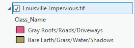
         Figure 7 to the right is the illustration that goes with figure 6. Each of the different types of land uses are very prominent and clearly visible. Thought this rough classification is not always completely correct it is what is used to figure out how much landowners will pay in regards to storm water fees. In figure 7 there is 7 land use types, the end goal is to get them into 2 land use types as shown in figure 9. To do this the reclassify tool was used and the impervious surfaces received a 0, while the pervious surfaces received a 1. Figure 9 shows a clear representation of whether or not the areas are Impervious or not impervious. The pink represents the roads, driveways and roofs, and the brown shows the bare earth, grass and shadows.

Figure 9

Figure 8

                   

                                                                                                                     Lesson 3

Figure 10

         In the third and final lesson the accuracy of the classifications in lesson two will be assessed by comparing it with the original image that was given. After it was determined that the data was accurate enough, there will be a calculated area of the impervious surface. The accuracy points are shown below in figure 12, they are 100 randomly generated accuracy points that are used to ensure the right type of land use is being identified. This was done using the create accuracy assessment points tool. The first ten points were gone through individually to make sure they are on what they say they are. Once the process was understood a master copy was available for use from ESRI in order to save time.

Figure 11

 

Figure 12

       Next came computing a confusion matrix that is shown to the left. To do this the confusion matrix tool was used and there is only an input and output available, the input was the Accuracy_Points and the output was placed in the Neighborhood_Data geodatabase and named Confusion_Matrix. The number in the bottom right corner of the table means that the data had a Kappa value of .92 that is the overall classification accuracy. A Kappa value of 85 to 90 should be re run because the data may not be accurate enough.















Results

          Figure 13 and figure 14 are two different maps that were derived from the aerial imagery that was processed using ArcGIS Pro. Figure 13 shows one of the end displays that shows what areas are impervious, as depicted by the brown and what areas are pervious, as depicted by the neon green. When looking at this alone a viewer would be able to tell that the area is a suburb. The lake is slightly unclear in figure 13, though it stands out really well in figure 14. Figure 13 is a good add on map to use with with other illustrations to help people to understand what areas absorb water and what areas do not.

Figure 13

   
          Figure 14 below clearly illustrates the differences in land use, this is done to give the viewer an opportunity to see what structures are in what places in relation to figure 13. Figure 14 clearly shows the lake in the center of the housing area. Then, breaking up the map into quadrants, there is an almost even distribution of structures or vegetation and each quadrant has a bit of water in it. There are a few large shadows denoted, that most likely are coming from trees. This is a good map to couple with figure 13 because the viewer will clearly be able to tell what is pervious and what is impervious.

Figure 14

Conclusion

         In closing, this lab was very informative and a really good beginning tutorial on how to use ArcGIS Pro. Aerial imgagery is very effective in finding out what areas are impervious and pervious to water. This was an important lab because what was done could be done by any city or government in an effort to better determine storm water bills. ArcGIS Pro online was much faster than expected and it looks to have a promising future in the geography field.


Sources

https://learn.arcgis.com/en/gallery/

https://learn.arcgis.com/en/projects/calculate-impervious-surfaces-from-spectral-imagery/

https://learn.arcgis.com/en/projects/calculate-impervious-surfaces-from-spectral-imagery/lessons/segment-the-imagery.htm

Processing Pix4D Imagery

Introduction

         Pix4D is used to change hundreds or even thousands of images taken from a Unmanned Aerial Vehicle to a geo referenced 2D or 3D display. This software aids in the construction of a point cloud data set, true orthomosaics and a digital surface model. This software can take skewed aerial images and change it to extremely accurate georeferenced mosaic. Images from aircraft can be uploaded as well, it is not strictly limited to just UAV. The images that will be used in this lab were collected by Joseph Hupy using a DJI Phantom 30 in 2016. The drone was flew over the Litchfield mine which is southwest of the city of Eau Claire, there are two data sets that will be getting used to complete this lab. Pix4D helps to generate maps from the aerial images, from there the maps can be disccused and dissected. Pix4D is a very powerful software that does have many applications and it can be used in many different settings. In an effort to understand what makes data qualified to be used in this setting a few questions must be answered first and they are displayed below. These questions help the Pix4D user understand how the UAV should be flown and also how to maintain data quality. This lab focuses on building maps with Pix4D, it is widely accepted as easy to use and it is the top of the line software. For this exercise there will be no GCP's (ground control points) used, and also there will be no oblique imagery, though the software does have the capabilities.

What is the overlap needed for Pix4D to process imagery?

          As a general standard there should be at least 75% frontal overlap in the flight direction and at least 60% side overlap between flying tracks. Also a constant height over the surface of the terrain helps to ensure data quality. There are exceptions to overlap, in densely vegetated areas there should be a 85% frontal overlap at least 70% side overlap, increased flight height can also help to make the aerial images appear not as distorted. An increased overlap and increased height ensures that the data will represent the terrain correctly.

What if the user is flying over sand/snow, or uniform fields?

          When flying over flat terrain with agriculture the user should have overlap of at least 85% frontal and at least 70% from the side and again flying higher can help improve the quality. When looking at unique cases such as sand or snow the user should have at least 85% frontal overlap and at least 70% side overlap. Also the exposure settings should be manipulated in order to have as much contrast as possible. Furthermore oceans are impossible to reconstruct because there is no land features. When flying over rivers or lakes the drone should be flew higher in order to capture as many land features as possible.

What is Rapid Check?
     
          Rapid check is made for use in the field, it can verify the correct areas of coverage and ensure that the data collection was sufficient. Rapid check is inside of Pix4D, it is not a stand alone software. The one downside of rapid check is that it processes the data so rapidly that it can be inaccurate. Rapid check should be used as a preview of the data in the field and the data should still be imported in the office when more time is available.

Can Pix4D process oblique images? What type of data do you need if so?

          Yes Pix4D can process oblique images, there needs to be many different angles and images of the oblique image in order to produce a quality data set. An oblique image is one that is taken when the camera is not straight up and down with the ground or the object. It is possible to combine oblique imagery with other kinds, for these cases there must be more overlap and it is recommended to use ground control points. According to the Pix4D site there should be an image taken every 5 to 15 degrees in order to make sure that there is a sufficient amount of overlap.

Can Pix4D process multiple flights? What does the pilot need to maintain if so?

          Yes Pix4D can process multiple flights, again the operator needs to ensure that there is enough overlap between the images taken in the flights.  When processing multiple flights it is important that the conditions were the same or at least nearly the same. To clarify there should be about the same cloud cover, the sun position should be taken into consideration and the overall weather will also play a role.

Are GCPs necessary for Pix4D? When are they highly recommended?

           Ground control points are not necessary for Pix4D, as long as there is adequate overlap there should not be any issues with flights that were taken perpendicular to the ground. If there is no image geo-location then the operator is strongly urged to use GCP's. Oblique aerial imagery can pose a few issues, when using oblique flight data there should be GCP's because they will help ensure that there was adequate overlap and that data integrity was not compromised.

What is the quality report?

          A quality report will be displayed after every step of processing. It will tell you if the processing failed or if it was completed. The report will tell the user if the data is ready to be worked with. The quality report runs a diagnostic on the images, dataset, camera optimization, matching and geo-referencing. This is essential because it makes sure the images have the correct amount of key points and ensures the image has been calibrated.

Methods

         The first step in this lab is to open Pix4D and start a new project. From here the project was named in a way that it can be told apart from other assignments. The numbers represent the year, followed by the month and lastly the day on which the project was started. Additionally the location the drone was flew and the type of drone and the height at which it was flown are all included in the name of the file. The name of the file ended up being 20170306_hadley_phantom50m, and this accounted for all of the information discussed above. Figure 1 below shows how and where the data was saved.

Figure 1

Figure 2

          From here the images were added from a folder that was provided by professor Joseph Hupy. The images from both flight 1 and flight 2 were added, though they were added separately in an effort to not bog down the computer.There was 68 images added from flight 1 and 87 images added from flight 2. Figure 2 above shows what the images appeared as after adding them from flight 1.

          Once the images were added it is important to take notice of the Coordinate system, though the default was used for this exercise it could have been changed. Also if the user ends up not being happy with the coordinate system once the data is in ArcGIS it can be changed. Next, under selected camera model in the edit tab it is important to make some changes. For whatever reason the Pix4D program has the Phantom 3 as being a global shutter, when in reality it is a Linear Rolling Shutter. All of the other camera specifications are correct.

          After clicking next there are options to change the processing options and the 3D map option was selected. Selecting the 3D map option means that Pix4D will create a Digital Surface Model (DSM). After selecting the 3D model and clicking finish, the map view will then be brought up. This gives the user a general idea of what the flight looked like. From here be sure to uncheck the boxes next to "point cloud and mesh" and the "DSM, Orthomosaic and Index." This is done so that it does not take hours to complete. Then by going into processing options in the lower left corner there are a series of processing options that can be changed to improve quality and speed. Under the "DSM, orthomosaic and index" tab the method was changed to triangulation. From past experiences this is the best option to select. From here the initial processing can be started. Once the initial processing is complete make sure the quality report is correct. Next, uncheck box 1 that says initial processing and select boxes 2 and 3 and process it again and again make sure the quality report is correct.

Figure 3

           Figure 3 above illustrates the steps discussed in the paragraph above. The number 2 and 3 boxes were unchecked to add in timely processing. At the time the screenshot was taken the software had just started running, it was only 5% complete with the first of 8 tasks. Figure 4 below shows the second time the data was ran for flight one, this time box 1 was unchecked and boxes 2 and 3 were selected.

Figure 4

           The quality report gives information on the accuracy and quality of the data, this is essential because it will tell the user if there were any errors in the data. The quality report shows a summary of the data, a quality check and also displays a map of the overlap. This shows that much of the data should have overlap of at least 4 images and this ensures the accuracy. Once flight 1 and flight 2 are both completed the images are now ready to be made into maps using ArcMap. The quality report is displayed below in figure 5. There is more to the quality report than what is displayed in the screenshot below, as the quality report is fairly lengthy.

Figure 5

          Figure 6 below is a part of the quality check, and it ensures that all of the images were calibrated and that the data was all accurate.

Figure 6

            Figure 7 below shows the name of the project, when it was processed and various other information.

Figure 7

           Figure 8 below displays the number of 2D keypoint matches. This also gives an idea of how accurate the data was and which areas may be slightly more accurate.

Figure 8

Results

          After the processing was completed a video was constructed using Pix4D in order to give the viewer an idea of the flight area. This does a fantastic job of giving a visual reference to the viewers. There is a lot of detail in the video due to the high resolution. A link for the video is posted below and the video is available to be viewed on youtube.

https://youtu.be/KRKbkdaLwUk

          Figure 9 is a screenshot of the area after the data was processed. It is extremely high resolution and it came out very nicely. This view was achieved by unselecting the camera, and then selecting the triangle mesh tab.

Figure 9

          After completion in Pix4D the data was then brought into ArcMap so a few maps could be made. The maps are displayed below as denoted by figure 10 and figure 11.

Figure 10

   

          Figure 10 above is a Digital surface model, overlayed with a hillshade of the Litchfield mine. The piles of sand are clearly visible by the bright red and the roads are depicted by yellow. This is an interesting map of something such as a mine because there are drastic elevation changes, much like the first sandbox activity that was completed this semester.

          Figure 11 below is a orthomosaic of the Litchfield mine that is located southwest of Eau Claire. The orthomosaic does a good job of showing what the mine is made up of. There are sand piles on the West side of the map and there is some vegetation more to the east. The main road runs in from the southeast and splits either left or right of the large sand pile that is located in the center. 

Figure 11

Conclusion

         As a final critique, Pix4D is a very good software for processing UAS data, it is very user friendly and it projected the data at a high resolution and was very aesthetically pleasing. Having never used the program before it only took the general outlined instructions provided in the powerpoint to be able to process data with Pix4D.
       

Sources

Pix4D Support
https://support.pix4d.com/hc/en-us/community/posts/203318109-Rapid-Check#gsc.tab=0