Ponds and Community Garden Near South Middle School Eau Claire

Introduction

        On Tuesday May 2nd was the first opportunity the class had to get out and see some UAV's in action. The DJI Phantom 3 advanced was flew first to collect the nadir images along with some oblique imagery of the students cars parked on site. Next, the DJI Inspire was flown to give the class an opportunity to try it out, no data was collected using that platform. This lab taught students how to collect GPS coordinates for the GCP's that were made in the previous lab. The GCP locations were collected using a $12,000 survey grade GPS and combined with the UAS data to increase spatial accuracy of the data.

Study Area

        Figure 1 below is a number of maps that show the study area for the data collection in this exercise. The area of interest (AOI) is located to the south of the Eau Claire South Middle School, just to the north of Pine Meadow Golf Course, and to the southeast of the corner of Mitchell Avenue and Hester Street. Data collection took place on May 2nd, and the conditions were partly cloud with a steady wind at 5mph with gusts up to 10-12 mph. In addition to the community garden area picture in figure 1, the ponds just to the south of the community garden was also flew.

Figure 1

Methods


         Figures 2, 3, and 4 below show a close up of the survey grade GPS that was used to obtain sub centimeter accuracy for this lab. The device is not hard to use, but there is a large amount of settings and useful features that do take some time to become comfortable with. The survey grade GPS was used to get a coordinate at sub centimeter accuracy, to be used with the UAS flight that was done a different day. The GCP's were created the week before the flights and the creation of them can be viewed in the previous blog. The GCP's that were previously laid out in the garden were left for this flight and the rest of the GCP's were spaced evenly across the road from the garden around the ponds. The survey grade GPS was again used to collect the coordinates for the GCP's. The coordinate system used was UTM WGS 1984 Zone 15N. After creating a new file for data collect the points of the GCP's can be collected by simply pressing one button.

Figure 2

       When using the survey grade GPS it is important to make sure that the level is accurate as pictured in figure 2 above. If the bubble is out of the circle it could hinder the data accuracy. After the data collection button was pressed it is essential to not move the GPS at all because the location will be altered then.

Figure 3

         Figure 3 above shows how the GPS unit was set up on the GCP's, it was carefully centered in the middle of the X before the data collection was started. Also the GCP's were collected in order from 1 to 16 to ensure that they were given the correct location when adding in the UAS flights.

Figure 4

        Figure 4 above is a close up of the screen that is attached to the shaft of the GPS unit, it is all pretty self explanatory to set up. Always be sure to check the coordinate system before data collection.

Figure 5

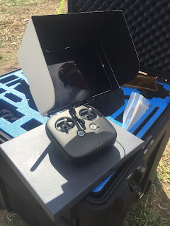
         Figure 5 above is the remote and tablet used to fly the DJI Inspire and figure 6 below is a picture of the DJI Inspire that was flown for fun and to get the class some experience flying.

Figure 6

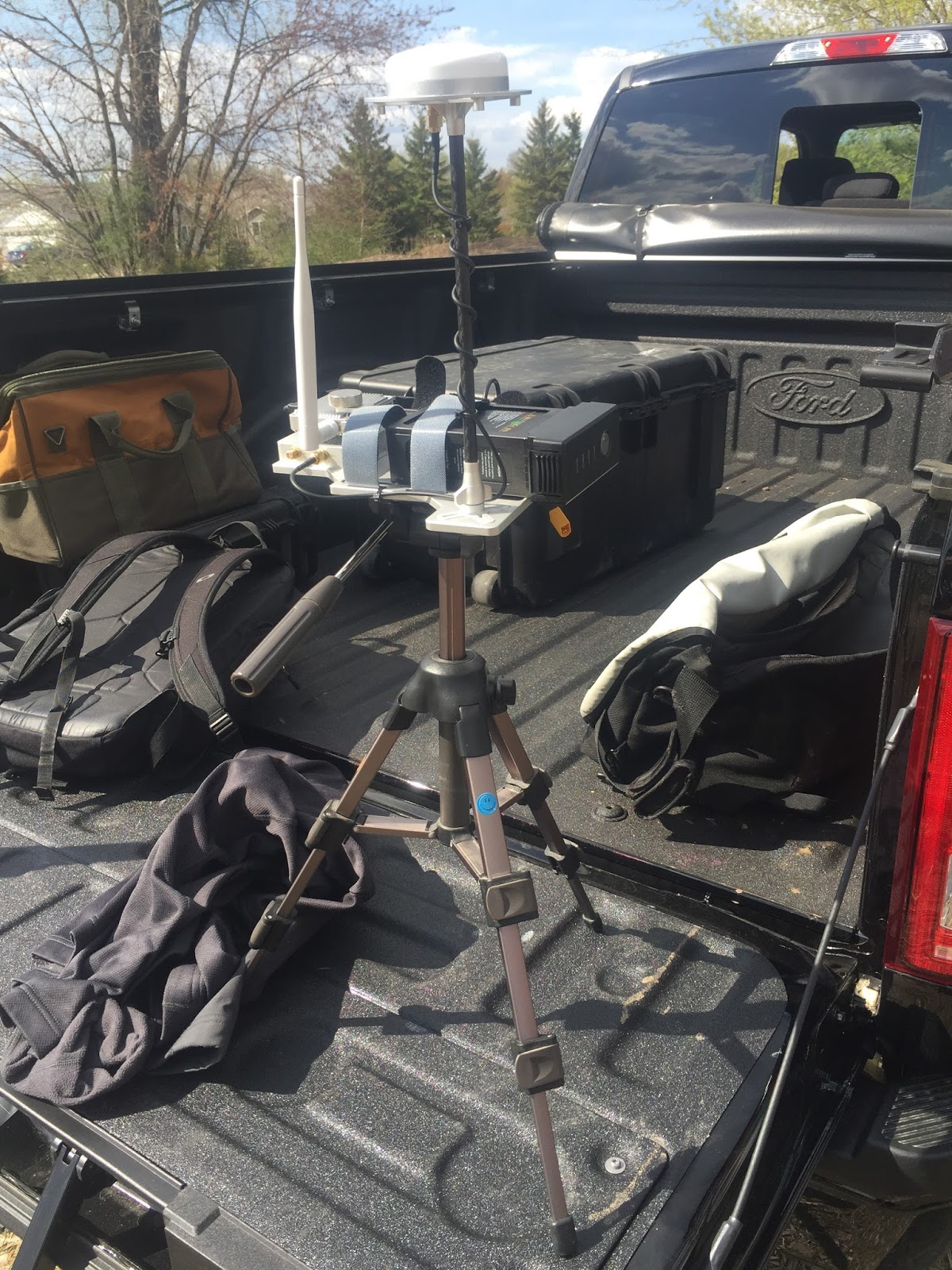
Figure 7

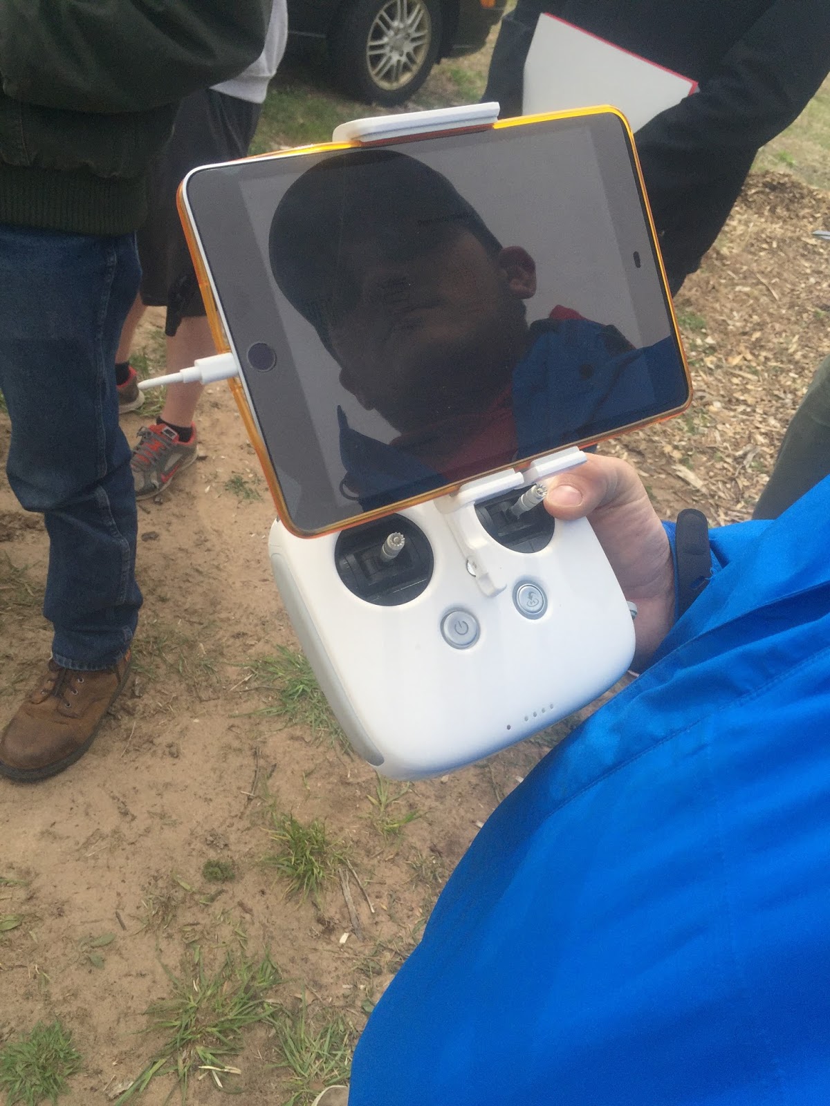
       Figure 7 above is the Real Time Kinematic (RTK) used in sync with the m600 to better data accuracy during the flight in real time. Figure 8 below shows the remote and the tablet used during the flight.

Figure 8

       Figure 9 below shows the DJI M600 used to generate the orthomosaic and DSM with hillshade that are pictured in figures 10 and 11.

Figure 9

Results

        Figure 10 below is an orthomosaic that was generated from the flight of the M600 over the garden and the pond to the south of South Middle school. The ortho is very high resolution and allows the viewer to get a good idea of the vegetation around the area. The image is very high resolution and the difference in the plot in the community garden should be noted. Also on the far right in the northeast corner, half of the left field of the baseball field is visible. The southern most pond is well over 6 times the size of the northern most pond.

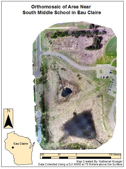Figure 10

        Figure 11 below shows a orthomosaic with a digital surface model and hill shade that was generated in ArcMap. This does a nice job of showing the changes in elevation throughout the area of interest. In the northeast corner the elevation is notably the highest, this makes sense because this is where the baseball and softball fields are located. The trail between the two ponds in the middle of the map shows that the trail is elevated in comparison to the ponds, obviously to make the trail passable. The ponds and the areas immediately around the ponds are a pretty dark blue, meaning that they are lower elevations than the majority of the rest of the map. To create the map below the transparency of the orthomosaic was set to 50% and the DSM was overlaid with the hill shade tab checked in ArcMap.

Figure 11

Conclusion

       In conclusion, it was a welcomed relief for the class to get out and do some real world flying and to then process the data after collecting it. The class created the GCP's, put them out, collected the GPS coordinates, assisted in the flight and processed the data, showcasing all of the skills that were learned throughout the semester. Over $20,000 dollars of equipment was used for this lab, showing that the class knows how to fly a number of different drones as well as how to operate the survey grade GPS for GCP coordinates collection.