Introduction
This lab was done almost identically to the previous lab, as it dealt with processing the same data in Pix4D, though this time there was an addition of ground control points (GCP's). The addition of GCP's helps ensure data integrity. In order to understand why GCP's are significant, they first need to be understood. Ground control points are a specific location on the earth's surface that was placed there by the operator flying the area in an effort to be able to tie images down to the earths surface. Each ground control point has a coordinate on the earths surface assigned to it. GCP's are used by drones, satellites, and airplanes and they are used to georeference the data that was taken during flight. As discussed in the previous lab, GCP's are not required when working with aerial imagery if the location of the images is known, but if the aerial images are not geolocated then GCP's must be implemented. Even when the images are geolocated they can still be off by tens of meters so the use of GCP's when possible is encouraged. In this lab a brief summary of running Pix4D will be discussed as well as the methods used to tie down the GCP's will be walked through. The initial processing will be re optimized after the GCP's have been tied down. In the end the goal is to determine the difference in data quality from aerial imagery with GCP's and aerial imagery without GCP's.
Methods
For this lab a new project was created in Pix4D, name the same way as the previous lab, except this time the GCP's were added to the end to show that GCP's were used. The initial directions for this lab instructed to run the Litchfield flights 1 and 2 separately. After running them separately there was issues with the merge and with the GCP's, most definitely user error, so the second time the flights were brought in together, which did add a significant amount of time to the process. Though this way took longer, there was no longer the step to merge and the data processed with no issues. In total there were 155 images brought into Pix4D. The steps in this lab were done almost identically to the previous lab. Be sure to change the camera mode to linear rolling shutter, as shown by figure 1 below. Next, under the "DSM, orthomosaic and index", which is tab 3, be sure to change the raster DSM method to triangulation rather than inverse distance weighting. The default coordinate system is acceptable for use here so leave that at WGS1984(egm96).
 |
| Figure 1 |
The next step is shown below by figure 2. Under the project tab, there is a GCP/ MTP manager that allows the user to import GCP's. After clicking on import GCP's the screen below will pop up, the coordinates order is changed to Y, X, Z rather than X, Y, Z because Y is the false easting, X is the false northing, and Z is the elevation. If it is left in X, Y, Z the GCP's will not import in the correct locations.
 |
Figure 2
 |
Figure 3
Figure 3 above shows where the images were taken from both flights 1 and 2. The blue X's mark the locations of the GCP's. All but 2 of the GCP's were tied down, for two of them they may have been moved or accidentally covered up. Before the initial processing was ran, the GCP's were tied down using the basic editor in order to make the initial processing more accurate and to make the later steps using the ray cloud easier.
|
|
 |
| Figure 4 |
After the initial processing was complete, the rest of the images were tied down using the rayCloud. Figure 4 above shows that the GCP's had to be tied down in every image they were visible in. This was done by zooming into the correct GCP and placing an "X" on the center. This is the process of georeferencing, using a point with a known coordinate to make the aerial imagery more accurate. After all of the GCP's were tied down for every image they showed up in, the imagery was then reoptimized.
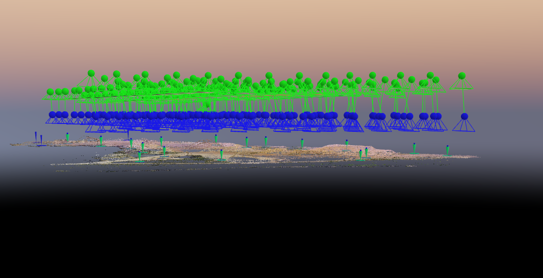
 |
| Figure 5 |
Figure 5 shows the imagery after reoptimizing for both flights 1 and 2. There was only 3 GCP's that remained blue and they did so because they did not show up in any of the images taken. As stated earlier this could be because they were moved, or accidentally covered up. The green points that are on the surface are the GCP's that were correctly tied down and reoptimized. After this step is complete, uncheck box 1 next to initial processing and check boxes 2 and 3 and press start. The final product of all the processing is a very high quality orthomosaic and DSM that can be used for map making in ArcMap.
 |
| Figure 6 |
 |
| Figure 7 |
Figure 6 and figure 7 above show a few snippets from the quality report that is received after processing. Figure 6 shows that 155 out of 155 images were calibrated and that there is georefrencing. The summary shows what the project was called and when the data was ran.
Results
In the results section there will be comparisons made between the Litchfield mine with GCP's and without. This will be done in an effort to determine if the GCP's are really worth the extra time. Figures 8-11 are maps generated from the aerial imagery that was processed in Pix4D, figure 8 and 10 are without GCP's and 9 and 11 are with GCP's.
 |
| Figure 8 |
Figure 8 shows a DSM overlaid with hillshade without GCP's and figure 9 illustrates the same things as figure 8 with the addition of GCP's.
 |
| Figure 9 |
In figure 9 it is easy to see the increases and decreases of elevation. The maximum elevation is just over 247 and that is shown by the dark red in figure 9. All of the sand piles show up nicely, for example in the southwest corner it is clear there is a substantial pile there. The lowest elevation points from the imagery are on the western side of the mine where it meets the east side of the water, this shows that the surface of the lake most likely has a lower elevation than the mine.
 |
| Figure 10 |
 |
| Figure 11 |
Figure 11 shows the Litchfield mine with GCP's, it is very accurate. The accuracy can be seen when looking at the shore line on the west side and also when looking at how well the roads line up on the east side of the map. It is so accurate that the roads line up perfectly with the imagery basemap that was added to the map.
Conclusion
After completing this lab there is no question that GCP's make data much more accurate though the differences did not really jump out at you. When looking at the orthomosaic, the difference is not that notable, other than a few small accuracy improvements it you look closely, as discussed in the results section. In contrast, the digital surface model (DSM) showed quite a large difference. What this should show someone working with aerial imagery is that GCP's are beneficial even though they are not required for use. Without question if the user was making maps from aerial imagery and getting paid for it, GCP's should be implemented.
Sources
Aerial Images provided by Dr. Joseph Hupy.
Pix4D Help
https://pix4d.com/support/


No comments:
Post a Comment